When I recently watched the Saturday afternoon football games of the first German Bundesliga (the highest league in Germany), I noticed something that I have been observing for many years. Players seem to get yellow cards on purpose to get suspended for the next away game. Why is that?

In a season, the yellow cards of each player are counted. If the player has received a total of 5 (red or yellow-red cards are not counted), he has to sit out a game. Receiving a 10th or 15th yellow card has the same consequence. For a player, it can make sense to get suspended on purpose to skip an unimportant match and save yourself up for the following matches. This practice is not 100% allowed, but it is hard to accuse the players of intention because yellow cards happen quickly, i.e., pulling the jersey, delaying the game, hard foul play. Furthermore, it is difficult to measure which games are essential for a single player (against the ex-club, against direct competitors, against top club), making it more complicated to blame someone.

However, another effect occurs: Players also seem to control whether they are suspended for an away or a home game. Having played amateur football for many years myself, I can confirm that players prefer to play at home, for rational reasons of long journeys, higher costs, etc. In order to find out whether this circumstance also plays a role for professional football players, I collected data, searched for anomalies, and examined the subject with a statistical hypothesis test.

Data acquisition

To gather the necessary data, I wrote a small script in Python and crawled the official website of the German Bundesliga:

Spieltag/Tabelle

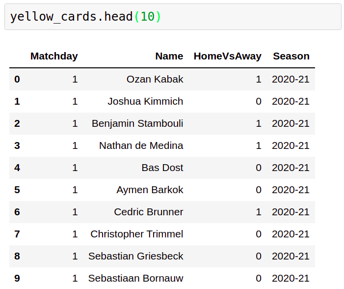
I retrieved all yellow cards from the last 7 seasons with additional information whether the card was given to the home team (0) or away team (1). In a follow-up blog post, I will describe in detail how I scraped the mentioned webpage to access the presented data. The processed data frame looks like the following:

To ensure the correctness of the data frame, I have tested random samples against manual counts. The data is available upon request!

Data presentation

As we have just seen, the information whether the yellow card is for the home or away team is encoded as 0 and 1 in the variable “HomeVsAway”. For example, the empirical distribution of received yellow cards for the home or away team in the 2020–2021 season can be easily obtained by taking the sum of the “HomeVsAway” column and dividing it by the total number.

Since 1 is encoded as “away”, we get a probability of ~50.9% that a randomly drawn yellow card was given to the away team in the season 2020–2021. In terms of probability distributions and random variables, we write:

Let us have a look at the empirical probability in each season:

We recognize that the trend continues over all seasons. If a player is in the away team, his chance is slightly higher to receive a yellow card over all seasons.

Clearly, it is visible that away teams tend to receive more yellow cards than home teams over all seasons. This might be due to the fact that home teams generally have more possession meaning the away team has to steal the ball more often which involves a higher risk to get a yellow card. Other guesses are that the referee is slightly on the home team’s side because of the support. Also, it can be assumed that the away team is more aggressive because they play against a whole stadium. Anyways, these are only speculations and no particular interest of this article.

In the next step, we compare the probability of getting a yellow card in an away game over all cards (1), over all 5th, 10th, and 15th cards (from now on, I will speak about 5th, but I mean all modulo 5) yellow cards (2), and for getting an idea about some other sample, also all 3rd yellow cards (arbitrary choice) are considered (3). To obtain this, we have to group by each individual player and count the number of yellow cards from the first matchday to determine if his 5th (or 3rd) card happened in an away or home game.

As seen in the plot, over all seasons, the black bars are almost always below the blue bars, which indicates a lower chance of getting the 5th yellow card in an away game than any other random yellow card. In the season 2015–2016, the chance of getting the 5th yellow card in an away game was the lowest.

If we compare the blue and the green bar, we see this effect being mixed for the 3rd yellow card. In this case, the probability is more or less equal to all seasons (sometimes higher, sometimes lower).

Despite the tendency in the data, we have to process a more objective method to decide if this is already significant.

Hypothesis testing

Null hypothesis: For any player, the chance of getting the 5th yellow card in an away game is as high as getting any yellow card in an away game.

In the following, we carry out four methods to test this hypothesis. At first, we repeat the experiment hundreds of times to estimate the p-value of accepting the null hypothesis according to the law of large numbers. Secondly, we will calculate the emerging empirical distribution analytically. The last two will be a t-test and Wilcoxon test conducted in python.

Law of large numbers

We have counted 604 5th yellow cards over all seasons, meaning 604 * 0.5277 = 319 yellow cards are expected to be given to the away team, according to the null hypothesis. In fact, according to the data, only 604 * 0.4701 = 284 yellow cards were given to away teams which deviates by 35 from the mean. To evaluate how realistic this deviation is, we simulate this experiment hundreds of times and calculate the proportion of experiments whose results deviate by 35 (two-tailed hypothesis test) or more.

The list “rounds” contains the outcomes of each simulation with 100, 1000, 10000 experiments for the number of 5th yellow cards received in an away game according to the null hypothesis (p = 0.5277). Calculating the p-value for each simulation gives us:

For n=100, there was not even one outcome deviated more than 35 from the mean. The law of large numbers tells us, the more experiments we conduct for a simulation, the more accurate is our final result. Our most accurate result is for n=10000 where we reject the null hypothesis with a p-value of 0.0043. To get a visual impression, we look at the empirical distribution of the simulation for n=10000:

Analytical approach

Also here, we apply a two-tailed hypothesis test. How likely is a deviation of 35 from the expected mean of 319? To do this analytically, we have to calculate an expected deviation from the mean. The list of yellow cards is a chain of Bernoulli trails — 1 (away) standing for “success”. Thus, the population size n enables us to calculate the expected deviation by

giving us a normal distribution that represents the probability of various numbers of yellow cards (#YCaway):

Calculating the area under the curve between the borders enables us to calculate the probability of getting a deviation of 35 or less from the mean of 319. Consequently, we receive a rejection probability (p-value) of

of this being happening under normal conditions. We notice that the analytical approach agrees very much with the outcome of the repeated empirical estimated p-values from above. Even the normal distribution looks very similar to the empirical distribution above for n=10000. If we simulate even more experiments, according to the law of large numbers, the p-value will converge towards the analytically obtained p-value.

In the following, I compare the results of the proportion of the 5th yellow cards and the 3rd yellow cards (as above in the bar plots) to get an impression of how the hypothesis test responds in both cases.

Using T-Test of scipy.stats:

The T-Test is used to compare two independent samples to test if the same generating process produced them. It focuses mainly on the mean values:

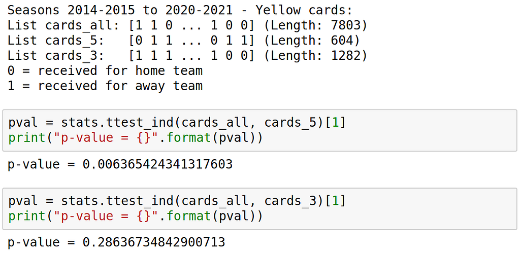
We receive a p-value of 0.006355 which strongly suggests that the 5th yellow cards are not generated by the same process as the rest of the yellow cards. We reject the null hypothesis. In the other example, we see by the p-value of 0.2864 that the 3rd yellow card very much agrees with the generating process. Here, we would accept the null hypothesis.

Using Wilcoxon signed-rank test of scipy.stats:

The Wilcoxon signed-rank is less susceptible to mean values and compares pairwise values.

We see that the Wilcoxon test assumes the null hypothesis for the 5th yellow cards only for p=0.03125, whereas for the 3rd yellow cards it assumes the null hypothesis for p=0.46875. Interestingly, the p-value is the highest here, but still not high enough to confirm the null hypothesis.

Outlook

In conclusion, the various statistical hypothesis tests have shown a change in the data when looking at the different yellow cards. Accordingly, when a player receives the 5th yellow card, the probability is significantly increased that it is more likely to take place at home than the rest of the distribution would suggest. This preference agrees with my own experiences as a former amateur player.
Moreover, I realize that the matches of a team do not always alternate (home, away, home, …), which is why this conclusion is somewhat doubtful. Nevertheless, it is the issue in most cases, and the significant differences were detected in the data, making this a fascinating insight. By the way, in the current season 2021–2022, the collected data until the 26th matchday suggests that the trend strongly continues by only having a 40.9% chance of getting the 5th yellow card as the away team:

Following this, one could still look at when the matches do not alternate making a future study more focused on the problem statement. In addition, one can check individual players to see whether there are candidates who deliberately operate this effect over the years.
In the end, I would like to point out that this study does not claim to be entirely valid, as it is only an on-the-side fun project. However, I wish to carry it out as accurately as possible therefore do not hesitate to contact me if you have found any mistakes or comments.