A year ago, my colleague and I embarked on a fascinating journey to uncover the mysterious behavior of our office blinds. We documented our initial findings in the article “Behavior of blinds: A sketch of scientific practice.” Since then, we have collected more data and refined our approach to analyze and predict the movement of the blinds. In this article, I will describe how I build an entire pipeline, from data collection to data and model visualisation, using Google Docs, machine learning models in Python, and a React-based website. The link to the website can be found in the Conclusion.

Data Collection and Preprocessing

The foundation of our project is the extensive dataset we have been collecting over the past two years. We continued to record the exact times the blinds went down, which we then stored in a publicly readable Google Doc. This method allowed for seamless collaboration and ease of access, as we could simply download the data once per day as a CSV file onto our server, avoiding the complexities of using the Google API.

As described in the previous article, it is important to note that the blinds do not go down every day, as their behavior depends on various factors such as sun, wind, brightness, and temperature. Even though we tried to capture these features, we could not see patterns that helped us improving our model. However, we found, if the blinds go down, they do not go down earlier than the fitted models suggest, indicating that the models serve as a lower limit for the blinds’ movement.

Before fitting the data to machine learning models, I preprocess it by removing any outliers. This step is crucial in ensuring that the models can effectively capture the underlying patterns without being influenced by irregular data points. One challenge during this preprocessing phase was transforming the date format into a more suitable format, such as integers (dates) or doubles (time), that could be easily read by the machine learning models. Then, I treated it as seasonal data that repeats each year. This involved mapping each day of the year to an integer value ranging from 1 to 365. These integer values, along with the year and the time when the blinds went down, were used as features for the machine learning models.

Machine Learning Models

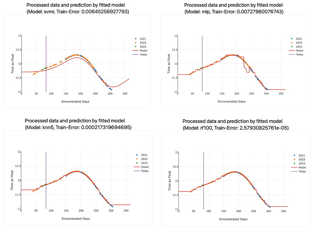
To predict the behavior of the blinds, I explored various machine learning models, such as k-Nearest Neighbors (k=2, 5 and 8), Support Vector Machine Regressor, Random Forest Regressor, and Multi-Layer Perceptron (Deep Neural Network). I trained these models on our preprocessed data and compared their performance in predicting the blinds’ movements.

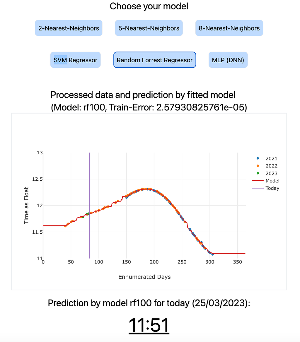
The input data for the models were integers ranging from 1 to 365, representing each day of the year. The output of the models is a double that is later mapped to a time of the day. After the models were fitted, they performed a prediction for each single day of the year (integers 1 to 365). The resulting doubles were transformed into times of the day using some normalization steps. These predictions for each input day and for each machine learning model were saved in a JSON file, which was then further processed by the React application. This allowed for an interactive and user-friendly visualization of the predictions, making it easier to understand the performance of each model and to compare their results.

The Random Forest Regressor shows the lowest training error, while the Multilayer Perceptron (DNN) and the Support Vector Machine Regressor exhibited the highest training errors. The k-Nearest Neighbors models can compete with the Random Forest Regressor. The training errors for each model are also displayed on the website. For a more sophisticated application, we would have split the data into training and testing sets to make our models robust against overfitting, but we wanted to keep the process simple, as the machine learning part is not the main focus of this project. Also, the models seemed to work quite well already.

I used Python and its vast ecosystem of libraries, including scikit-learn for machine learning, pandas for data processing, and numpy for other numerical computations, to implement and evaluate the different models. With the models fitted to the data, I could predict the lower limit if the blinds would go down on any given day. The prediction of the current day is displayed on the website.

Visualising the Results with React

The React application including Tailwind for the styles provides an interactive and user-friendly way to visualize (using Plotly) the predictions generated by the various machine learning models. The input data for the plots are stored in JSON files, which are the output of the pre-trained machine learning models. These JSON files contain the predictions for each day of the year and are updated daily.

It is important to note that the models’ results presented on the website are pre-trained each day and do not undergo a new training process when the user clicks the button to view the predictions. Instead, the React application retrieves the pre-trained model predictions from the JSON files and displays them in the form of interactive plots. This approach allows for a seamless user experience and ensures that the website remains responsive and efficient, without the need for time-consuming model training on each user interaction.

The use of React, combined with the pre-trained model predictions, offers an effective way to visualize and compare the performance of the various machine learning models, enabling users to gain insights into the behavior of the blinds and assess the accuracy of the predictions.

Automating the Process

To ensure our predictions are always up-to-date, I automated the entire process. Every day, our server downloads the data from the publicly available Google Doc as a CSV file, fits the machine learning models, and saves the results as JSON files. This approach ensures that our models stay relevant as new data points are added, allowing for continuous improvement in our predictions and our application.

The automation is conducted using a cronjob on my Linux server, which is a virtual server rented from the provider Strato. It has its own IP address and is permanently accessible. The cronjob is configured in the file /etc/crontab on the server. A screenshot of the crontab configuration is provided can be seen in Figure 2. The Apache2 web server is used to host the website on the Linux server.

Conclusion

Through the combination of Google Docs, machine learning models in Python, and React with Tailwind, I have managed to create an end-to-end pipeline that not only uncovers the hidden patterns in our office blinds’ behavior but also visualises the results in an engaging and interactive manner. Surprisingly, implementing the machine learning models was relatively easy and fast compared to the rest of the pipeline. This project does not necessarily focus on the machine learning part but on an end-to-end application. This also emphasises the critical role of data. In today’s world, models are easily replaceable and trainable, but even the most advanced models cannot compensate for a lack of quality data.

In a tongue-in-cheek manner, this project highlights the power of interdisciplinary collaboration and draws parallels with the scientific process, where researchers often delve into the most minute details of a narrow and tiny subfield. In the end, it serves as a light-hearted reminder that, much like science itself, we can sometimes lose ourselves in the pursuit of knowledge, even if it involves understanding the seemingly pointless behavior of office blinds.

The website is accessible on https://christophsaffer.com/apps/blinds.