In the last season 2023/2024 of the German cup in football, the so-called “DFB-Pokal”, a team from the 3rd league, 1. FC Saarbrücken, made it to the semi-finals. Not only does this seem to be a rare event, but they also eliminated three Bundesliga clubs in previous rounds. By the semi-finals, Bayer Leverkusen was the only remaining Bundesliga team. But how rare or unlikely is it really? How are the chances between first league and lower league teams distributed? Using a stochastic model simulating each single game of the DFB Pokal per round with dedicated win probabilities, we are trying to explore these questions.

Data acquisition

Before going more deeply into the model architecture, we have to acquire data about the results in the German cup over the last years and design a meaningful structure (data model) that can serve for the stochastic model. To achieve this, I created an automated Python script to scrape data from the webpage fussballdaten.de, collecting team information from each round of the DFB Pokal over the past 20 years. The DFB Pokal is a knockout tournament starting with 64 teams each year. The teams from the first (18 teams) and second (18 teams) Bundesliga are predetermined. The remaining 28 teams vary and are a mix of teams from the third league and the winners of regional cups (can also be third league and lower). To estimate each team’s strength better, we did not only save the league of each team, but also the league position in the end of the season.

But why do we want to save the league position of the single teams? This is because, we can not assume a uniform distribution regarding their “strength” across all teams of one league, i.e. Bayern Munich won the DFB Pokal much more often than any other first league team. On the other side, there is simply not enough data available to estimate the winning probabilities between each teams from each league and league position. Therefore, we have to use simplified assumptions to reduce the parameter space and introduce categories, based on league position and league itself. These are:

• 1: First league teams from position 1–6
• 2: First league teams from position 7–12
• 3: First league teams from position 13–18
• 4: Second league teams from position 1–9
• 5: Second league teams from position 10–18
• 6: Third league teams
• 7: Everything below

The resulting dataset looks as follows:

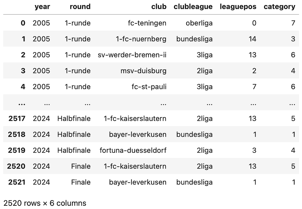
Please note that we did not save results of single games but only the information which team made it to which round per year. The variable “clubleague” is categorical and has four options (bundesliga = first league, 2liga = second league, 3liga = third league, and oberliga = everything below 3 league). The variable “leaguepos” is an integer and reflects the position in the league in the end of the season. In case no information was found (mainly for teams in “oberliga), then the script inserted “0”. The variable “category” is the variable derived from clubleague and league position to reduce complexity.

Data processing

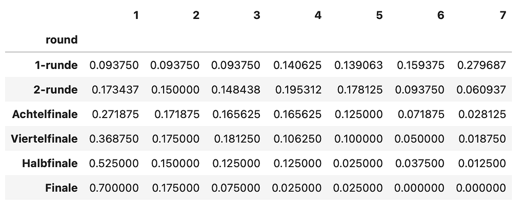
We can now use this dataset to perform frequency counts and generate a new dataset that represents the likelihood of each team, based on its category, reaching a specific round:

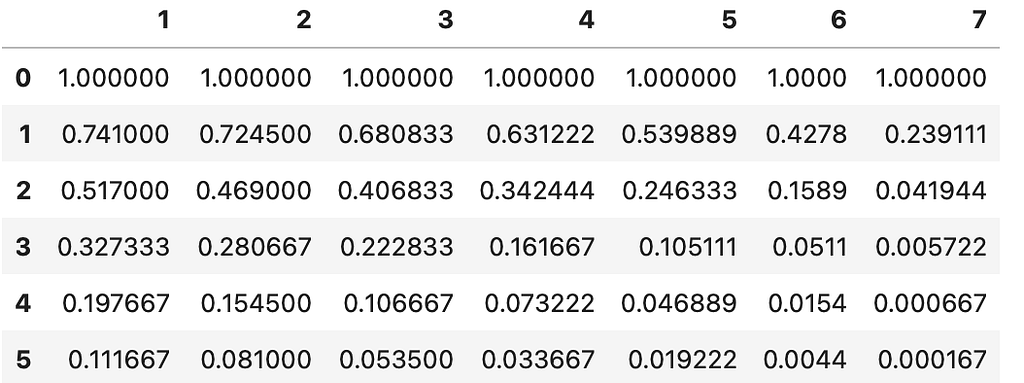
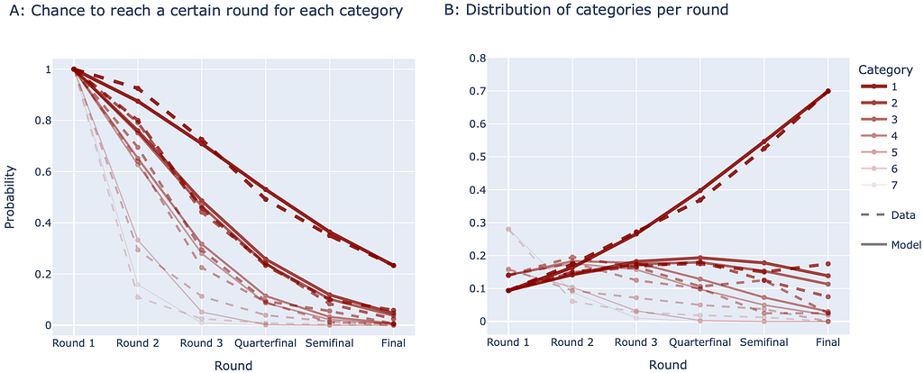
Here it becomes clear why cateogories are necessary. There is simply not enough data to estimate the probability for each league position per league. Also the probabilities between close-by teams is nearly the same, which is a point to reduce complexity. What else can we see? For example, for a first league team in the positions 1 to 6, the chances to reach the final is about 23%. Positions 7 to 12 or 13 to 18 only have 5.8%, respectively 2.5% chance. The second league teams (categories 4 and 5) only reach about 0.6% while for lower teams it is impossible (according to the last 20 years). In addition, we can also look at the percentual composition of each round per category:

In this figure, we can recognise that 70% of the teams in the final were from the first category (first league, positions 1–6). These two datasets in Figure 2 and 3 serve as ground truth data to which the stochastic model will be fitted.

Stochastic model for win probabilities

To simulate an entire knockout tournament of the DFB Pokal, the process to decide which team wins and goes to the next round had to be modeled. To do this, I created an array, clubs, with 64 elements, where each index (0 to 63) corresponds to a specific league and position, i.e. clubs[63] represents the team from the first league at league position 1. With the index of each club, their specific score (the higher, the better) can be represented and accessed in an array for win probabilities win_probsto derive the probability between two teams. Let’s have a look at an exemplary distribution for the array win_probs:

In this example, the teams at indices 0 to 17, which are in the category 7 have a score of “1”, while the first six team of the first league, indices 58 to 63 have a score of “13”. In the model, the win probability between two teams is calculated as:

P(“Team i wins against Team j”)=clubs[i]/(clubs[i] + clubs[j])

For example, based on the distribution in Figure 4, if team 63 plays against the team 0, then its win probability is (13/(13+1)) = 93%. If team 55 plays against team 50, then its win probability is 11/(11+9)) = 55%. Using this model, we can simulate the knockout tournament and try different distributions for the array win_probs, run it multiple teams to generate average results and compare them with the data in Figure 2 and 3. The program used to run the model simulations is structured as follows:

The parameters of the model are encoded in the array ps which are the scores of the single categories from which the probabilities between the categories are derived. If we run this model, we receive the following results for the probabilities of a team to reach a respective round (compare Figure 6 to the data in Figure 2 — and Figure 7 to Figure 3):

As we can see, the prediction is not very accurate. For example, it underestimates the category 1 and generally does not reflect the data. This can also be measured using the sum of squared error (SSE) between the data (Figures 2, 3) and the prediction (Figures 6, 7), reaching here a SSE of SSE=0.54. To find the optimal set of parameters, have to minimize the SSE.

Parameter estimation

To estimate the optimal set of scores in the array ps and reduce complexity, the boundaries of the score system have to be determined. For this, we set p1=p[0]=1, and try to find out the maximum value for p7=p[6]. This can be done by looking into the approximate probability of “oberliga” teams playing against top 6 teams in the first league. As we did not save the single results per match, we manually went through the last 20 years. As it is quite a sensation when a lower league team wins against a top 6 first league team, these events were quite accessible and we came to a result of lower than 1% of the matches end in favor of the lower league teams. Therefore, we set the score for p[6]=p7=999. With this, there are five more parameters to estimate as we have: ps=[1, p2, p3, p4, p5, p6, 999]. Also, we assume that there is an order of the parameters, as usually teams in higher leagues and higher positions are stronger: 1 < p2 < p3 < p4 < p5 < p6 < 999.

For the estimating the remaining parameters, several options are available which should not be part of this article here and might elaborated in a follow-up article. However, due to the stochastic nature of the model, we obtain a parameter distribution (known as a posterior distribution) from the estimation algorithm, rather than fixed parameter values. The results of these distributions look as follows:

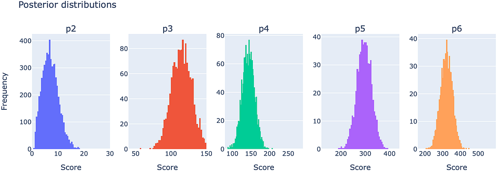
We receive the following parameters, based on the pre-set parameters and the mean values per distribution: ps=[1.0,6.6,116,142,298,322,999]

What does these parameter tell us? Clearly, they show that the top 6 teams in the first league (Score: 999) are by far more successful than the rest of the teams. Also, the remaining categories for first league (Scores, 322 and 298) are closer to each other than for the second league (Scores 116 and 142), meaning there is quite a difference between first and second league instead of first teams in the second and last teams in the first league. From these parameters, we can compute a symmetric matrix and see the win probabilities between the categories:

Per row, the matrix shows the win probabilties against the respective category. For example the first row says that teams from category 1 win with 50% against their own category, with 78.5% against category 2, 77.7% against category 3, and so on. If we simulate the stochastic model with these parameter values, we receive a low SSE=0.045. Also the results can be visualised comparing the model predictions to the data in Figure 2 and 3 that we collected:

Parameter interpretation & predictions

The fitted parameter represent a score from 1 to 999 from which win probabilities can be calculated. What do the single values tell us? For example, there is not such of a big difference between Oberliga (Category 7, Score: 1) and 3rd league (Category 6, Score 6.6). However, if we go to second league (Categories 5 and 4, Score 116–142), and even to first league (Categories 3, 2, 1, Score > 298), the scores reach high values, showing that the jump from 3rd to 2nd, and from 2nd to 1st league are quite large in quality. In addition, the jump to becoming a top 6 team is tremendous (Score 999) and also indicates why one of these big teams usually win knockout tournaments (world cups, the euro, …), not because there are so many, but just because their chance of winning is significantly higher. The lower in the leagues we go, the broader the quality of the teams become.

Using this stochastic model, we can also run exemplary simulations. For example, assuming we have a tournament with only one top 6 team (Category 1, Score 999) and 63 middle class teams from the first league (Category 2, Score 322), our simulations show that the chance is still 20% that this one top 6 team would win the tournament.

We can also simulate conditioned events, meaning we start the tournament at a certain round under a given constellation of teams. For example, in the last season 2023/2024, something interesting happened. In the quarterfinals, there were only three teams left from the first league (Leverkusen, Stuttgart and Gladbach), while the only two remaining top 6 teams were even playing against each other (Leverkusen vs. Stuttgart). In contrast, according to our data in Figure 3, around 6 teams from the first league can be expected in the quarterfinals. Our conditioned simulations show that the chance, that one of the two remaining top 6 teams playing against each other (Leverkusen or Stuttgart) would win the tournament, was already at around 75%. On the contrary, considering that the other remaining first league team (Gladbach) played against Saarbrücken (Oberliga) in the quarterfinals, the chance of winning the tournament for them was “only” at about 20%, because these top 6 teams are so difficult to eliminate.

Conclusions

Overall, a model is presented that reflects the dynamics of the knockout tournament of the German cup, the “DFB-Pokal”. We could derive scores of the single team categories and estimate win probabilities. It shows that the top 6 teams are overly dominant while the team quality broadens when going to lower leagues. The model is a reduced representation of the available data and could be used to estimate win probabilities for certain scenarios. Here, one should be aware that the calculated results generally are only forecasts for larger sample sizes while the outcome of a single game is difficult to predict. In general, to make this approach more sophisticated, several follow-up steps can be done:

• Experimenting with the number of categories (clusters) or even use an unsupervised learning algorithm to find the clusters automatically
• Use different model approaches and designs acknowledging the varying performance (scores) during one season
• Scrape more data for the real results of each game to verify derived probabilities (scores)
• Scan for more data of different countries / competitions

In this regard, while the approach still has potential and could benefit from a more in-depth analysis, the emerged stochastic model represents a good starting point and can provide valuable insights.